Sensitivity Trendline Analysis Window
This window is used to set the different variables to calculate the trendline in your data to be able to do the sensitivity assessment. Simply follow the steps through the window menu at the top (see figure).
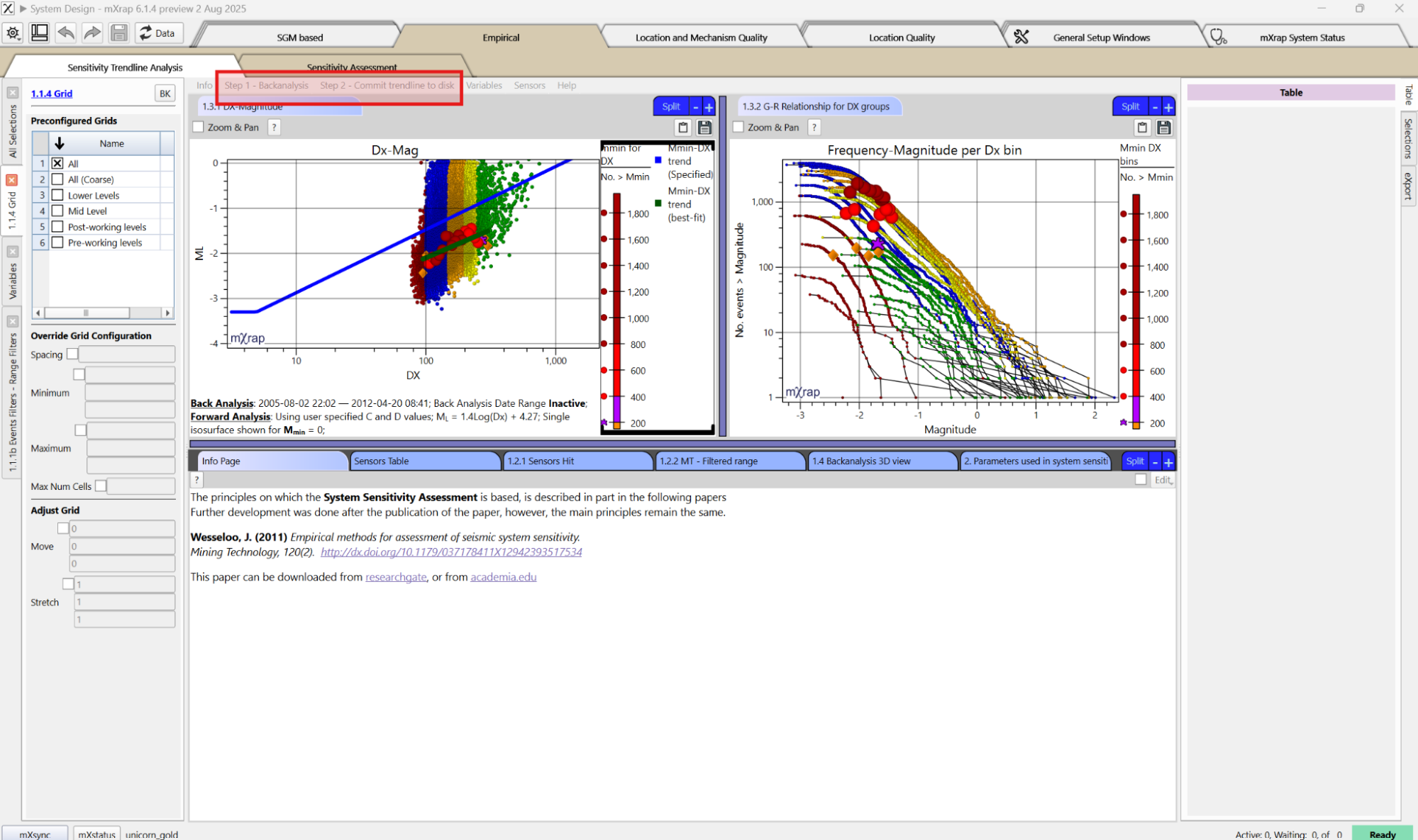
Each tool holds the step number in the title to help guide you through the process.
1.1 Choose data to work with
The first step is to decide which events to use and select your grid.
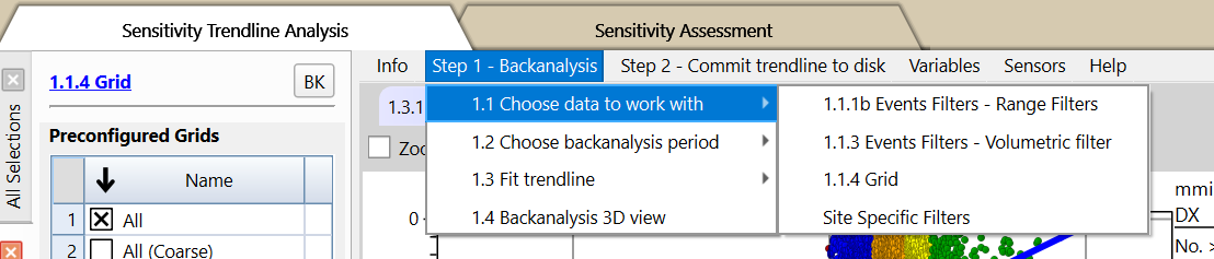
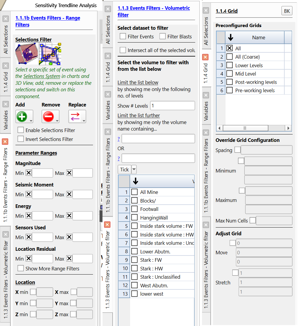
Steps 1.1.1b and 1.1.3 are filter panels that allow to filter the events based on ranges, selection boxes or volume filters. Step 1.1.4 is the Grid panel where the grid to be used for the analysis is selected. If you don’t have any grid set up, please click here to find how to.
1.2 Choose backanalysis period
The next step is to select the backanalysis period that will be considered.
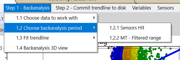
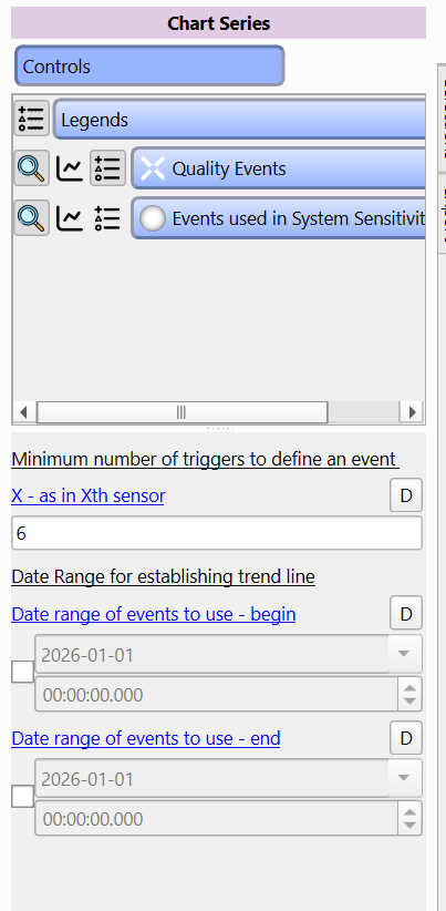
There are two charts to help with deciding the backanalysis period: the Sensors Hit vs Time (step 1.2.1) and Magnitude-Time graph (step 1.2.2). For the sensor hit chart, the minimum number of triggers to define an event can be modified in the Controls panel of the chart.
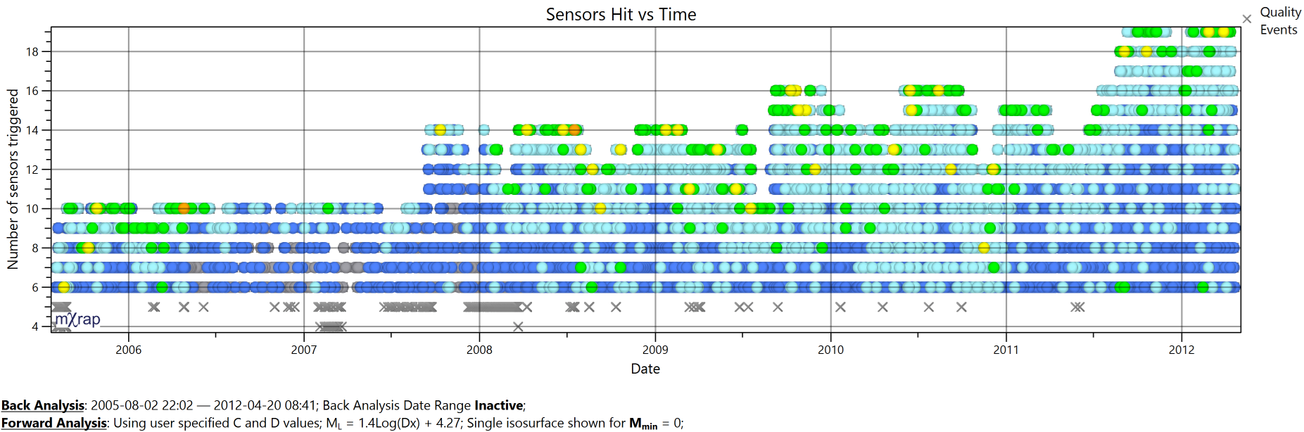
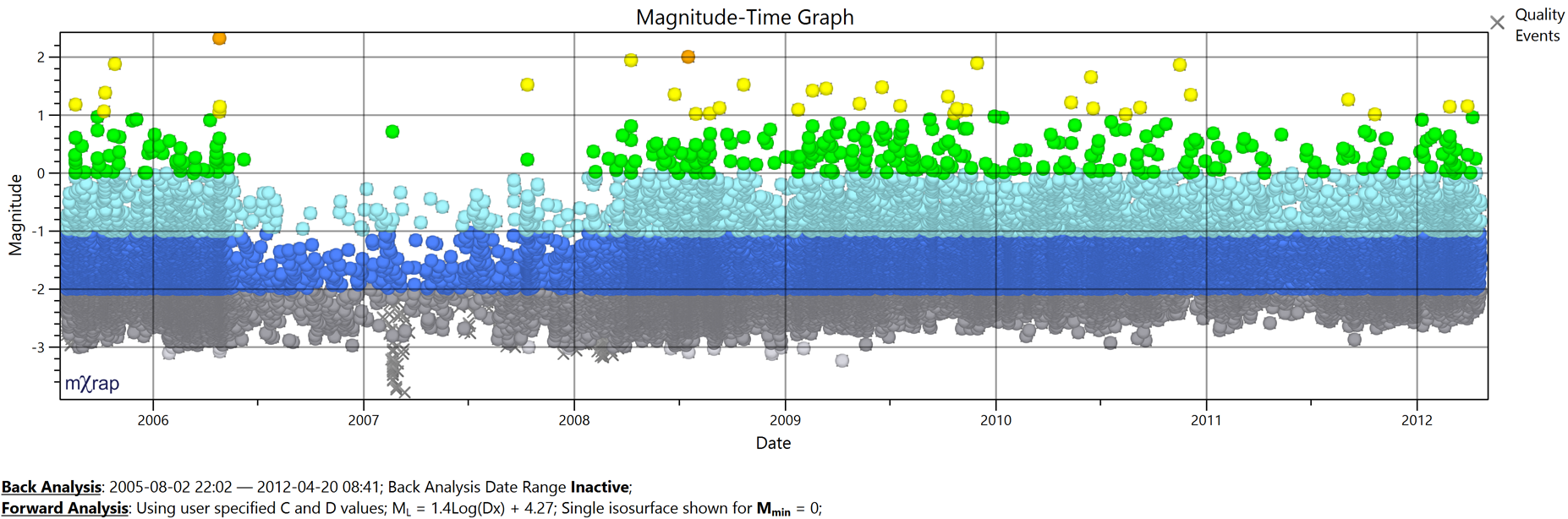
The selected time period can be set in the control panel of either of the two charts or in the Variables panel.
1.3 Fit trendline
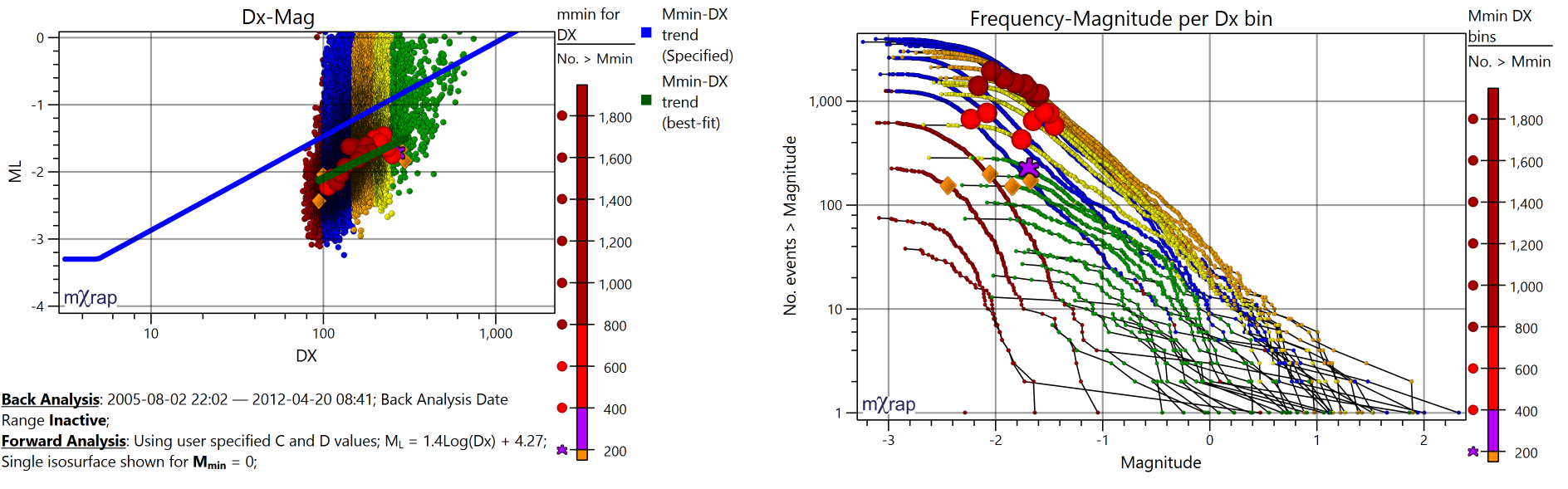
The next step is to fit the trendline that will be used to calculate the sensitivity on the selected grid. The trendline will be automatically fit based on the previous step selections and on the fitting variables. The trendline is plotted in the Dx-Mag chart (step 1.3.1) and the Mmin per groups are plotted in the G-R relationship for Dx groups chart (step 1.3.2). Each chart's variables are in their respective Controls panels. They can also be found in the Variables panel.
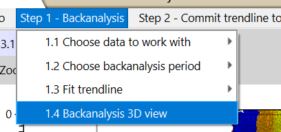
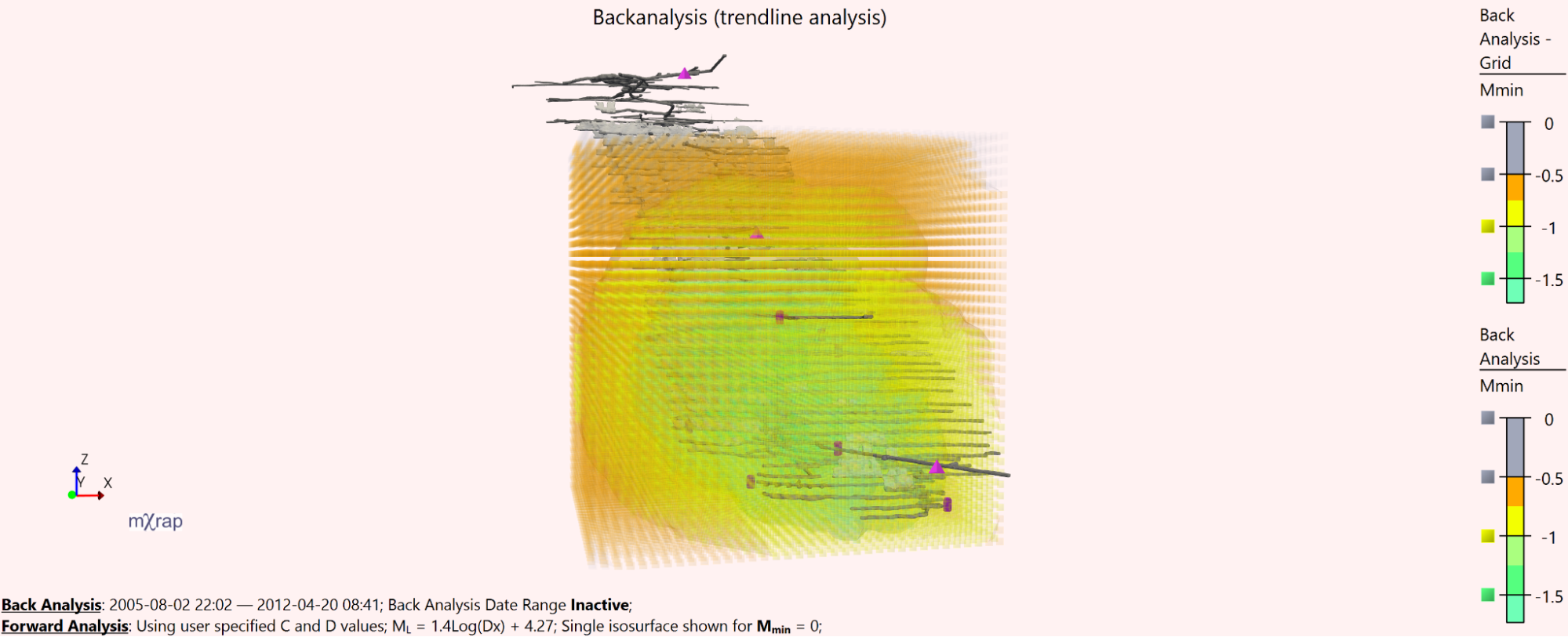
1.4 backanalysis 3D view
The next step is visualising the results in the 3Dview. The Mmin can be plotted per grid point and using ISO surfaces.
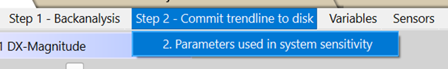
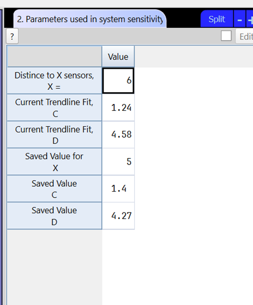
2. Commit trendline to disk
The final step is to save the trendline information for sensitivity assessment.
The table displays the current values for the number of sensors (X) selected and the trendline fit (C and D) as well as the saved values. If the values differ, the table can be edited and the saved values updated.
Additional tools in the window
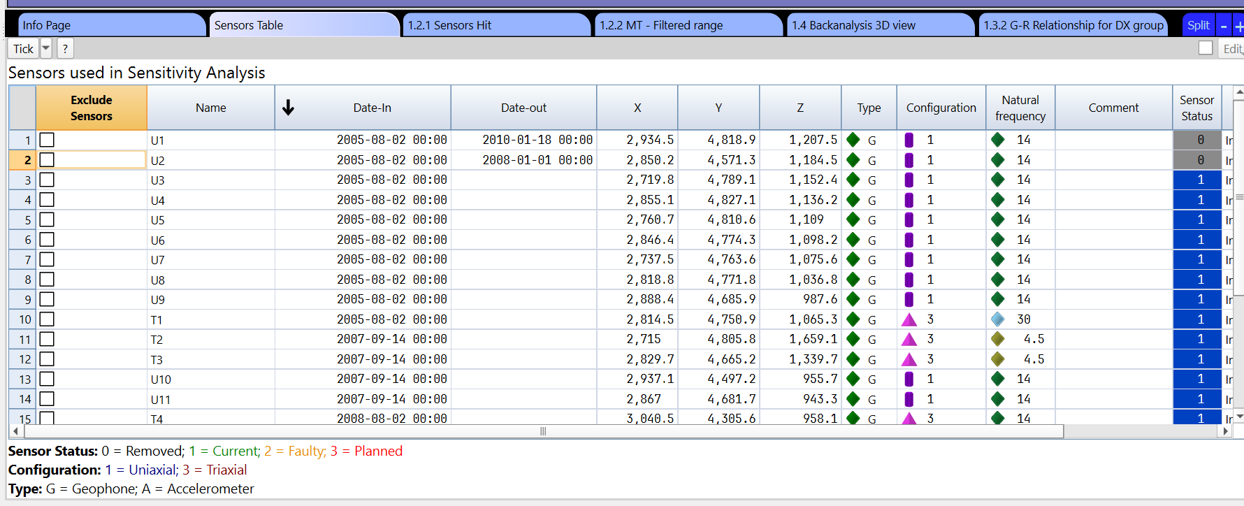
There is a Sensors Table where sensors can be excluded when doing the backanalysis set up.
There is a Sensor Pick panel that allows visualising sensor information based on the sensor picked in the 3D view using the F2 key.